The Taguchi Method in Quantisweb Methodology
M’Hammed Mountassir Ph.D. Quantisweb Technologies Inc.
Introduction:
This article demonstrates how the Quantisweb methodology, which combines aspects and approaches of three areas of Applied Mathematics: Decision Theory (AHP approach: Analytical Hierarchical Process), Statistics, and Optimization Techniques; is applied in the context of a Taguchi design industrial type of problem. The comparison study demonstrates that Quantisweb is applicable when the Taguchi method is applicable and it demonstrates that it is even more applicable because Quantisweb methodology uses multidimensional loss functions, with weighted optimization that achieves robustness in fewer experiments.
Background:
Design of experiments allows for better planning of experiments in scientific research and industrial studies. Design of experiments is applied in numerous disciplines and in industries where experimenters wish to quantify the relationships between functions of interest (response functions) y1,….,yp and variables (factors) x1,….,xk.
If the protocols adapted to design of experiments are followed, the maximum amount of information can be obtained with the minimum number of experiments [1], [2], [3]. A design of experiment is considered complete if all the experiments from all the permutations of the levels of all the factors involved are done. For example, if there are 7 factors and each one allows 2 levels, then the complete factorial design consists in doing 27 = 128 experiments. But generally, only a fraction of this number is done, which is called fractional design [4]. In the case of two-level factors, several methods have been developed, in particular those of Plackett and Burman [5], in which the number of experiments required is either 4, 8, 12, 16, 20, 24. These methods allow experimenters to make factorial designs intermediate to those of fractional factorial designs, which allow for only 4, 8, 16, 32 experiments. After the Second World War, when resources were scarce and financing was at its lowest, a Japanese engineer named Genichi Taguchi [6], [7], [8] put forward a method called Robust Design, to help engineers in the automobile industry during the product design phase, the phase in which gains in quality are the most significant, with the aim of reducing costs. In the Oriental mindset, the person who prevents a breakdown from happening is valued more than the person who makes a repair in record time!
In this article, Taguchi’s technique will be briefly discussed, and with an example of data, a comparison will be made with Quantisweb methodology [9].
The Taguchi Method:
In his approach to total quality, G. Taguchi took up the concept of design of experiments to develop a new method to help master this quality in product design. Starting in the 1970s, this method was introduced in Europe and the United States. It was vulgarized, and tables of combinations of practical experiments were published. It is necessary to try to analyze the ideas that Taguchi brought to the industrial world to understand how he could convince some users while being criticized and considered controversial by others. His approach was very interesting because by touching on the problem of the quality of a product in its totality, from its design to its end use, he developed a rationalization and philosophy of quality. This is no doubt why he was so original en comparison with the traditional attitudes of statisticians, who so often deal with short-term solutions. Chemists dealing with phenomena involving a large number of factors were to be heavy users of the Taguchi method.
To present a summary of the evolution of Taguchi’s techniques, we must explain his basic philosophy and his notable contribution to the improvements of quality control.
The methodology emphasizes the functional variation of a major property of the product which can play a role in the product’s performance such as pressure, response time, time between breakdowns. This methodology centers on three major points:
Loss function:
This stipulates that if one knows the ideal value (Id) that one wants variable Y to attain, then based on Taylor’s development of Y in the neighborhood of (Id), Taguchi was able to come up with a mathematical model in which the loss function is a quadratic function in two forms, either the loss function associated with the non-quality of the product : Q(y) = L(y-Id)2 where L = a constant or by modeling the variable of interest in the form : Y = μY + ε where μY is the average of the random variable Y that Taguchi calls the signal and ε is the random error variable of the model supposed with mean zero and variance σ2, that he calls noise. In this case the average loss function is approximately equal to: Q(y) = L[(μY – Id)2 + σ2]. To minimize this average loss, one must act on the factors that act on the signal to minimize (μY – Id)2, and act on the factors that act on the noise to minimize the variance σ2.
Orthogonal arrays and linear graphs:
As was mentioned, Taguchi classifies the factors the influence the product over its lifetime, and not only when it leaves the factory, in four categories:
– Controlled manufacturing factors that influence the signal μY, which we will note as x1i
– Controlled manufacturing factors that influence both the signal μY and the noise σ2, which we will note as x2i
– Uncontrollable factors that influence the signal, which we will note as z1i
– Factors whose influence is not certain, which we will note as z2i
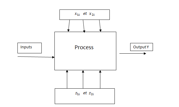
z2i factors are often disregarded. We can therefore see the signal as a function of (x1i ,x2i) and noise as a function of (x1i ,x2i). Two situations may then occur: Either reliable determinist models are available to model variable of interest Y as a function of these factors (as is the case in problems in physics or electrical circuits) and then the study of the variations of the signal and noise can be done by simulation. Or we do not have determinist relations and then experimental studies allow us to statistically hypothesize a model for the signal and a model for noise. Taguchi thus adapted orthogonal arrays (developed by Fisher to control experimental error) to determine the variation of the variable around the average. For every level of a factor, all the levels of the other factors are produced the same number of times.
The construction is based on three principles:
– Use only a limited number of tables, chosen per their particular properties.
– Make these tables easy to use through linear graphs.
– Consider interactions of order two or more as negligible.
By way of example, if we construct a Taguchi table associated with a design of experiment of 4 factors, A, B, C, and D, each having two levels, we will obtain the following table:
| A | B | AB | C | AC | BC | D | |
| E1 | 1 | 1 | 1 | 1 | 1 | 1 | 1 |
| E2 | 1 | 1 | 1 | 2 | 2 | 2 | 2 |
| E3 | 1 | 2 | 2 | 1 | 1 | 2 | 2 |
| E4 | 1 | 2 | 2 | 2 | 2 | 1 | 1 |
| E5 | 2 | 1 | 2 | 1 | 2 | 1 | 2 |
| E6 | 2 | 1 | 2 | 2 | 1 | 2 | 1 |
| E7 | 2 | 2 | 1 | 1 | 2 | 2 | 1 |
| E8 | 2 | 2 | 1 | 2 | 1 | 1 | 2 |
With this table, we have 8 degrees of freedom distributed as follows:
- 1 degree to estimate the overall average effect
- 1 degree to estimate the effect of A, one for the effect of B, one for the effect of C, and one for the effect of D.
- The three others to estimate the effects of AB, AC, and BC.
But Taguchi uses controllable factors as well as uncontrollable noise factors; he uses crossover designs, allowing us to minimize the number of combinations of these two types of factors to be done. For example, in the case of 3 controllable factors (C1, C1, C3) and three uncontrollable factors (N1, N1, N3) each having two levels (+, -), the crossover design will look like this:
| N1 | – | + | – | + | |||
| N2 | – | – | + | + | |||
| N3 | + | – | – | + | |||
| C1 | C2 | C3 | |||||
| Run1 | – | – | + | Y11 | Y12 | Y13 | Y14 |
| Run2 | + | – | – | Y21 | Y22 | Y23 | Y24 |
| Run3 | – | + | – | Y31 | Y32 | Y33 | Y34 |
| Run4 | + | + | + | Y41 | Y42 | Y43 | Y44 |
Therefore 16 experiments must be done, 4 repetitions for each of the 4 experiments required with controllable factors. If the number of controllable factors is equal to 7 and if the number of uncontrollable factors remains equal to 3, all of them having two levels, then a minimum of 32 experiments must be done.
Robustness:
For the product as well as the manufacturing process. The robustness of the product is to be taken in the sense that the influences of the changes in non-controllable operating factors are minimal. The robustness of the manufacturing process is to be taken in the sense that the end product undergoes minimal effects caused by changes in non-controllable operating factors. To minimize loss due to the non-quality of the product, Taguchi proposes using the ratio of signal over noise, which is generally noted as SN or S/N, to optimize his crossover plans, and thus four different criteria are generally implemented per the nature of the response function and its ideal value (Id):
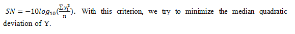
- The smaller the better: This criterion is used when the ideal value is nil, and takes the following form:
- The larger the better: This criterion is used when the ideal value is infinite. It takes the inverse form of the preceding:

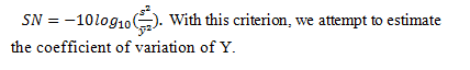
- The closer the better: This criterion is used when the ideal value is finite and not nil. It takes the following form:

- When the response function is binary: The following function is used:

In an optimization study, which uses Taguchi methodology, we try to maximize the SN ratio because a maximization of this criterion is equivalent to minimizing the loss functions. Since the purpose of this article is to make a comparison of the Taguchi method and Quantisweb methodology, we will consider a case where both methods are applicable.
Case study comparing the Taguchi method and Quantisweb methodology:
To understand the methodology in detail, please refer to article [9] on the Quantisweb website www.quantisweb.com This complete integrated method allows users to have an optimal combination of all the factors used simultaneously, with only a number of required experiments equal to the number of factors plus one. The method is centered on 3 principles:
- The A.H.P multi-criteria method of Saaty [10]
- Multidimensional statistical modeling
- Optimization techniques with or without constraints.
This case is based on the article by H. B. Wang & al: « Optimizing Multiple Quality Characteristics by Taguchi Method and TOPSIS Algorithm » published in The International Journal of Organizational Innovation, Vol 4 Num. 2 (2011) [11]. First we will apply the Taguchi method, and then we will do two simulations with Quantisweb methodology.
Taguchi method:
We have considered 8 factors at 3 levels, except the first, A, which has only two levels, as indicated in the following table:
| Factors /Levels | 1 | 2 | 3 |
| A. Antioxidants | 2.9 | 3 | |
| B. Synthetic plastics | -5 | 2 | 10 |
| C. Stabilizer | -0.1 | 0 | 0.1 |
| D. Lubricants | 0.8 | 1 | 0.2 |
| E. Flow auxiliary | -0.1 | 0 | 0.1 |
| F. Thickening agent | -0.1 | 0 | 0.1 |
| G. Compounding temp. | -10 | 10 | 30 |
| H. Compounding time (min) | 2 | 4 | 6 |
According to the suggestions of the technical department, three characteristics of the product have been taken into consideration: RI (Residual Induction), SG (specific Gravity) et MAF (Magnetic Attraction Forces). The following table summarizes the experiment data:
| A | B | C | D | E | F | G | H | RI | SG | MAF | |
| E1 | 1 | 1 | 1 | 1 | 1 | 1 | 1 | 1 | 56.37 | 8.35 | 16.78 |
| E2 | 1 | 1 | 2 | 2 | 2 | 2 | 2 | 2 | 56.39 | 8.60 | 13.49 |
| E3 | 1 | 1 | 3 | 3 | 3 | 3 | 3 | 3 | 56.22 | 8.47 | 16.52 |
| E4 | 1 | 2 | 1 | 1 | 2 | 2 | 3 | 3 | 56.17 | 8.36 | 16.26 |
| E5 | 1 | 2 | 2 | 2 | 3 | 3 | 1 | 1 | 56.62 | 8.45 | 17.95 |
| E6 | 1 | 2 | 3 | 3 | 1 | 1 | 2 | 2 | 56.84 | 8.63 | 17.84 |
| E7 | 1 | 3 | 1 | 2 | 1 | 3 | 2 | 3 | 56.73 | 8.56 | 17.73 |
| E8 | 1 | 3 | 2 | 3 | 2 | 1 | 3 | 1 | 56.58 | 9.21 | 17.95 |
| E9 | 1 | 3 | 3 | 1 | 3 | 2 | 1 | 2 | 56.92 | 8.63 | 18.17 |
| E10 | 2 | 1 | 1 | 3 | 3 | 2 | 2 | 1 | 56.95 | 8.42 | 18.99 |
| E11 | 2 | 1 | 2 | 1 | 1 | 3 | 3 | 2 | 56.47 | 9.07 | 18.49 |
| E12 | 2 | 1 | 3 | 2 | 2 | 1 | 1 | 3 | 56.61 | 8.85 | 18.69 |
| E13 | 2 | 2 | 1 | 2 | 3 | 1 | 3 | 2 | 56.71 | 8.60 | 17.79 |
| E14 | 2 | 2 | 2 | 3 | 1 | 2 | 1 | 3 | 55.93 | 8.47 | 15.85 |
| E15 | 2 | 2 | 3 | 1 | 2 | 3 | 2 | 1 | 56.98 | 8.65 | 18.89 |
| E16 | 2 | 3 | 1 | 3 | 2 | 3 | 1 | 2 | 56.24 | 8.78 | 19.65 |
| E17 | 2 | 3 | 2 | 1 | 3 | 1 | 2 | 3 | 56.81 | 8.69 | 18.06 |
| E18 | 2 | 3 | 3 | 2 | 1 | 2 | 3 | 1 | 56.64 | 8.69 | 19.37 |
Using the Taguchi method and the TOPSIS algorithm, the authors determined the optimal values of the parameters and the corresponding values of the characteristics of the product. In the following table, the optimized values obtained are compared with the current product data.
| Factors / Levels | SN ratio | ||||||||||
| A | B | C | D | E | F | G | H | RI | SG | MAF | |
| The research method | 2 | 3 | 3 | 2 | 2 | 2 | 2 | 1 | 58.195 | 14.014 | 13.21 |
| Current level | 1 | 2 | 2 | 2 | 2 | 2 | 2 | 2 | 56.66 | 0.0756 | 12.30 |
Quantisweb Methodology:
Since there are 8 factors, we used 9 trials out of the preceding 18. Quantisweb methodology is a complete integrated method, so it requires that the optimal values desired for each of the characteristics be specified. Therefore, two simulations with different ideal values were done. The results are summarized in the following two tables:
- Case where the ideal values are 50 for RI, 8 for SG and 10 for MAF.
| Factors / Levels | SN ratio | ||||||||||
| A | B | C | D | E | F | G | H | RI | SG | MAF | |
| Quantisweb OPV | 2.93 (2) | -5 (1) | 0.1 (3) | 0.8 (1) | -0.1 (1) | -0.1 (1) | 17.58 (close to 2) | 6 (3) | 56 | 8 | 16.6 |
- Case where the ideal values are 60 for RI, 10 for SG and 20 for MAF.
| Factors / Levels | SN ratio | ||||||||||
| A | B | C | D | E | F | G | H | RI | SG | MAF | |
| Quantisweb OPV | 3 (2) | 13 (3) | -0.1 (1) | 1.2 (3) | 0.1 (3) | 0.1 (3) | 30 (3) | 2 (1) | 57.05 | 9.66 | 18.47 |
It can be seen that in each of the cases, Quantisweb methodology gives us optimal values of the parameters that enable us to get as close as possible to the ideal values of each of the properties of the product, simultaneously. Quantisweb methodology is very flexible in comparison with the Taguchi method because it is not necessary to transform data into the signal-noise ratio, and even more importantly, regardless of the number of non-controllable factors, all that has to be done is add them to the controlled factors, and the number of required trials is always equal to the total number of factors plus one, no matter how many levels they have.
Conclusion:
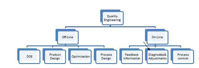
In this article, we have described the Taguchi method, which is based on robustness as a means of neutralizing the effects of uncontrollable factors called noise. This robustness is achieved using four types of estimation functions of the signal-noise ratio depending on the ideal value of each of the characteristics. The example of data confirms that Quantisweb methodology can be applied when the Taguchi method is applicable. Even more so because Quantisweb methodology uses multidimensional loss functions, with weighted optimization per the importance of each of the characteristics of the product around the ideal value specified by the user. Quantisweb methodology is part of a very vast field of optimization and quality control at all stages of problems of formulation (including mixture problems [12] where Taguchi is not applicable) or design and control of a manufacturing process, as can be seen in the visual below. We do not wish to get into a futile debate between statisticians and engineers over the adequation of this or that method. Our goal is not to stir up controversy over different methodologies but instead to give users different tools to allow them to get the maximum out of each one.
References:
[1] BoxG.E.P., Hunter W.G., Hunter J.S. “Statistics for experimenters’’ second edition, John Wiley & Sons (2005).
[2] Montgomery D.C. “Design and analysis of experiments’’ 7th edition Wiley (2011).
[3] Kettaneh W. & al “ Design of experiments: Principles and applications’’ 3rd edition, Umetrics Academy (2008).
[4] Vijay N. “Fractional designs’’ Department of Statistics and Industrial Operations Engineering. Michigan University (1995).
[5] Plackett R.L., Burman J.P. “The design of optimum multifactorial experiments’’ Biometrika, no 33 (1946).
[6] Glen S.P. “Taguchi Methods: A Hands-On approach’’ Addison-Wesley publishing. (1993).
[7] Taguchi G., Subir C., Yuin W. “Taguchi’s Quality Engineering Handbook’’ John Wiley & Sons (2004).
[8] Taguchi G., Subir C., Taguchi S. “ Robust Engineering’’ MC Graw-Hill (1999).
[9] Mountassir. M. “Quantisweb Methodology’’ (2006) White paper MDM Technologies Inc.
[10] Saaty. T. L. “ The Analytic Hierarchy Process, Planning, Priority Setting, Resource Allocation’’ Mc Graw-Hill (1980).
[11] Wang H.B & al. “ Optimizing multiple quality characteristics by Taguchi method and TOPSIS algorithm’’ The International Journal of Organizational Innovation.’’ Vol 4 n0 2 (2011).
[12] Mountassir, M. “Mixture Design & Quantisweb methodology’’ (2009) White paper MDM Technologies Inc.